Chapter 7 Generalized Linear Models (Binomial)

7.1 Students dataset

We want to analyze how students choose the study program from general, academic and technic (vocation)

ses: socio-economic status
schtyp: school type
read, write, math, science: grade/score for each subject

library(readr)
# load the data
# tsv - similar format to csv
students <- read_delim("./datasets/students.tsv", delim = "\t", col_types = cols(
  id = col_double(),
  female = col_factor(),
  ses = col_factor(),
  schtyp = col_factor(),
  prog = col_factor(),
  read = col_double(),
  write = col_double(),
  math = col_double(),
  science = col_double()
))

# or with RData file
load("./datasets/students.RData")
head(students)

## # A tibble: 6 × 9
##      id female ses    schtyp prog      read write  math science
##   <dbl> <fct>  <fct>  <fct>  <fct>    <dbl> <dbl> <dbl>   <dbl>
## 1     1 female low    public vocation    34    44    40      39
## 2     2 female middle public vocation    39    41    33      42
## 3     3 male   low    public academic    63    65    48      63
## 4     4 female low    public academic    44    50    41      39
## 5     5 male   low    public academic    47    40    43      45
## 6     6 female low    public academic    47    41    46      40

7.2 EDA

As usual, a bit of data exploration before performing any statistical analysis.

# count the occurrences of all classes combinations (in prog and ses)
with(students, table(ses, prog))

##         prog
## ses      vocation academic general
##   low          12       19      16
##   middle       31       44      20
##   high          7       42       9

# using students dataframe attributes,
# call the rbind function using as arguments
# the result of the tapply operation,
# that is three vectors with mean and sd for the
# levels of `prog`
#
# the result is a 3x2 dataframe with mean and sd
# of the two columns
with(students, {
  do.call(rbind, tapply(
    write, prog,
    function(x) c(m = mean(x), s = sd(x))
  ))
})

##                 m        s
## vocation 46.76000 9.318754
## academic 56.25714 7.943343
## general  51.33333 9.397775

# or, with dplyr
library(dplyr)
library(reshape2)

## 
## Attaching package: 'reshape2'

## The following object is masked from 'package:tidyr':
## 
##     smiths

students %>%
  group_by(prog) %>%
  summarise(mean = mean(write), sd = sd(write))

## # A tibble: 3 × 3
##   prog      mean    sd
##   <fct>    <dbl> <dbl>
## 1 vocation  46.8  9.32
## 2 academic  56.3  7.94
## 3 general   51.3  9.40

# simple way: do this for every program
mean(students$write[students$prog == "general"])

## [1] 51.33333

7.2.1 Plots

Boxplots allow to have a view of the distribution of a numeric variable over classes in a minimal representation. It shows first, second (median) and third quartiles, plus some outliers if present.

# boxplot in R
boxplot(students$write ~ students$prog)

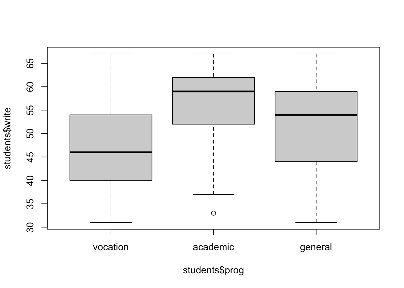
# precise boundaries (numbers) are found with the `quantile()` function
with(students, {
  quantile(write[prog == "vocation"], prob = seq(0, 1, by = .25))
})

##    0%   25%   50%   75%  100% 
## 31.00 40.25 46.00 53.50 67.00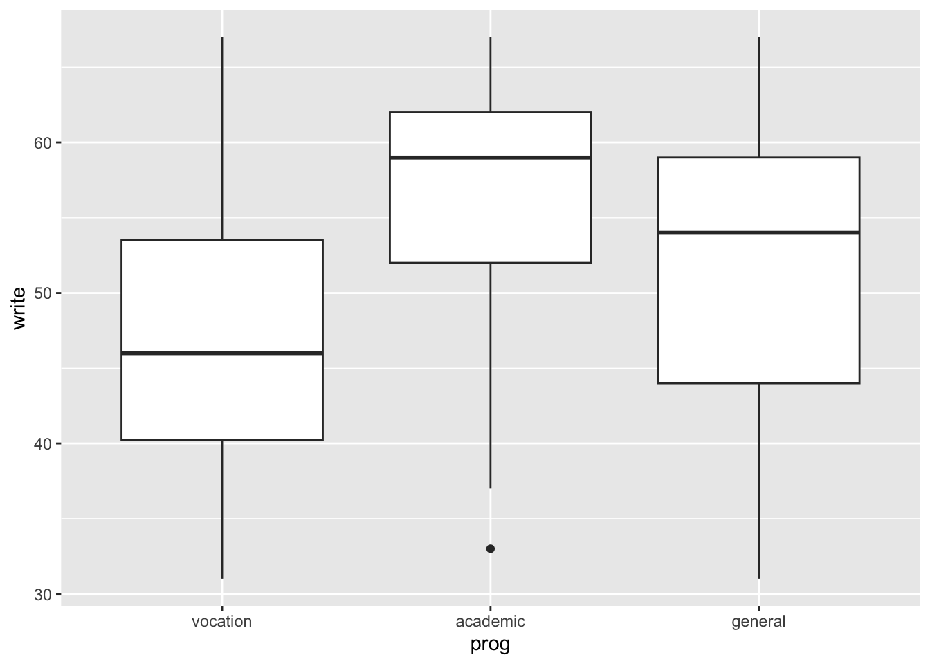

# boxplot in ggplot
library(ggplot2)
students %>%
  ggplot(aes(prog, write)) +
  geom_boxplot()

# geom_violin() # try also the "violin plot"

We can also put all subjects together, but we need to switch to long format with gather (or reshape2::melt).

# view of the grades distribution depending
# on subject and program
students %>%
  gather(key = "subject", value = "grade", write, science, math, read) %>%
  ggplot() +
  geom_boxplot(aes(prog, grade, fill = subject))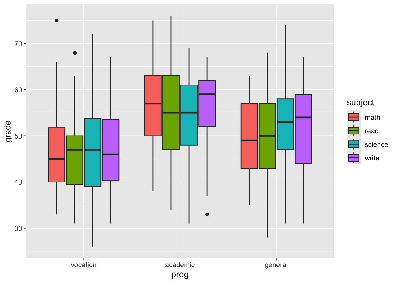

# or in different plots with
#    ...
#    geom_boxplot(aes(prog, grade)) +
#    facet_wrap(~ subject) # instead of

7.3 Test

We can further analyse the dataset attributes with some tests and traditional linear regression fit.

with(students %>% filter(prog != "vocation"), {
  tt_wp <- t.test(write[prog == "general"], # are the two prog distributed the same way?
    write[prog == "academic"],
    var.equal = TRUE
  )
  lm_wp <- summary(lm(write ~ prog)) # lm with qualitative predictor
  anova_wp <- summary(aov(write ~ prog)) # anova
  list(tt_wp, lm_wp, anova_wp)
})

## [[1]]
## 
##  Two Sample t-test
## 
## data:  write[prog == "general"] and write[prog == "academic"]
## t = -3.289, df = 148, p-value = 0.001256
## alternative hypothesis: true difference in means is not equal to 0
## 95 percent confidence interval:
##  -7.882132 -1.965487
## sample estimates:
## mean of x mean of y 
##  51.33333  56.25714 
## 
## 
## [[2]]
## 
## Call:
## lm(formula = write ~ prog)
## 
## Residuals:
##     Min      1Q  Median      3Q     Max 
## -23.257  -4.257   2.705   5.743  15.667 
## 
## Coefficients:
##             Estimate Std. Error t value Pr(>|t|)    
## (Intercept)   56.257      0.820  68.610  < 2e-16 ***
## proggeneral   -4.924      1.497  -3.289  0.00126 ** 
## ---
## Signif. codes:  0 '***' 0.001 '**' 0.01 '*' 0.05 '.' 0.1 ' ' 1
## 
## Residual standard error: 8.402 on 148 degrees of freedom
## Multiple R-squared:  0.06811,    Adjusted R-squared:  0.06182 
## F-statistic: 10.82 on 1 and 148 DF,  p-value: 0.001256
## 
## 
## [[3]]
##              Df Sum Sq Mean Sq F value  Pr(>F)   
## prog          1    764   763.7   10.82 0.00126 **
## Residuals   148  10448    70.6                   
## ---
## Signif. codes:  0 '***' 0.001 '**' 0.01 '*' 0.05 '.' 0.1 ' ' 1

Notice how the T-test t-value is equal to the linear model coefficient estimate t-value. They are computed the same way.

7.4 Generalized Linear Model

The \(X\)s have to be independent, thus we check the correlation plots.

library(GGally)
students %>%
  dplyr::select(math, science, write, read) %>%
  ggpairs(progress = FALSE)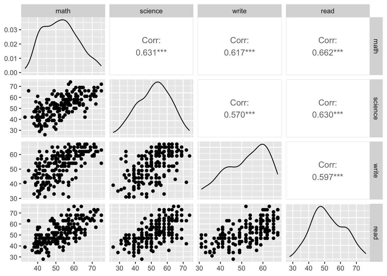

In order to be able to use the Binomial generalized linear model and set the program as response variable, we have to make a new dataset in which we define a binary class instead of a three levels factor. Here we arbitrarily choose to create a variable which is 1 for vocation and 0 for general.

# create a new dataframe
students_vg <- students %>%
  filter(prog != "academic") %>% # make distinction vocation-general only
  mutate(vocation = ifelse(prog == "vocation", 1, 0)) # transform class to binary

voc_glm <- glm(vocation ~ ses + schtyp + read + write + math, # choose some predictors
  data = students_vg, family = "binomial"
) # fit glm with binomial link

# new pipe operator (base R 4.2 or later) allows to send
# pipe results to any function parameter (not just the first one)
# and it's compatible with lm/glm calls (no need to create new datasets)
voc_glm <- students |>
  filter(prog != "academic") |>
  mutate(vocation = ifelse(prog == "vocation", 1, 0)) |>
  glm(vocation ~ ses + schtyp + read + write + math,
    data = _, family = "binomial"
  )
# `_` is placeholder for the piped dataframe

summary(voc_glm)

## 
## Call:
## glm(formula = vocation ~ ses + schtyp + read + write + math, 
##     family = "binomial", data = students_vg)
## 
## Coefficients:
##               Estimate Std. Error z value Pr(>|z|)  
## (Intercept)    3.78961    1.62184   2.337   0.0195 *
## sesmiddle      1.04148    0.53206   1.957   0.0503 .
## seshigh        0.42122    0.68145   0.618   0.5365  
## schtypprivate -1.06617    0.87344  -1.221   0.2222  
## read          -0.02558    0.02940  -0.870   0.3843  
## write         -0.02011    0.02836  -0.709   0.4782  
## math          -0.04175    0.03438  -1.214   0.2246  
## ---
## Signif. codes:  0 '***' 0.001 '**' 0.01 '*' 0.05 '.' 0.1 ' ' 1
## 
## (Dispersion parameter for binomial family taken to be 1)
## 
##     Null deviance: 131.43  on 94  degrees of freedom
## Residual deviance: 118.24  on 88  degrees of freedom
## AIC: 132.24
## 
## Number of Fisher Scoring iterations: 4

In the summary output, few differences from the lm call can be noticed:

the p-value for each coefficient is determined through a z-test instead of an exact t-test;
R-squared cannot be computed (there are no residuals) and the deviance is printed instead:
- Null deviance represents the distance of the null model (which has only the intercept) from a “perfect” saturated model
- Residual deviance compares the fit with the saturated model (with number of parameters equal to the number of observations)

We can do the same thing with the pair academic/general.

students_ag <- students %>%
  filter(prog != "vocation") %>%
  mutate(academic = ifelse(prog == "academic", 1, 0))

academic_glm <- glm(academic ~ ses + schtyp + read + write + math, # same predictors
  data = students_ag, family = "binomial"
)
summary(academic_glm)

## 
## Call:
## glm(formula = academic ~ ses + schtyp + read + write + math, 
##     family = "binomial", data = students_ag)
## 
## Coefficients:
##               Estimate Std. Error z value Pr(>|z|)    
## (Intercept)   -5.07477    1.47499  -3.441 0.000581 ***
## sesmiddle      0.23316    0.47768   0.488 0.625471    
## seshigh        0.77579    0.54950   1.412 0.158004    
## schtypprivate  0.61998    0.53668   1.155 0.248007    
## read           0.02441    0.02793   0.874 0.382069    
## write          0.01130    0.02753   0.411 0.681416    
## math           0.06720    0.03164   2.124 0.033689 *  
## ---
## Signif. codes:  0 '***' 0.001 '**' 0.01 '*' 0.05 '.' 0.1 ' ' 1
## 
## (Dispersion parameter for binomial family taken to be 1)
## 
##     Null deviance: 183.26  on 149  degrees of freedom
## Residual deviance: 157.94  on 143  degrees of freedom
## AIC: 171.94
## 
## Number of Fisher Scoring iterations: 4

Of course, we get different coefficient estimates with different models. We can compare them:

cbind(
  summary(voc_glm)$coefficients[, c(1, 4)],
  summary(academic_glm)$coefficients[, c(1, 4)]
)

##                  Estimate   Pr(>|z|)    Estimate     Pr(>|z|)
## (Intercept)    3.78961265 0.01945937 -5.07476526 0.0005805405
## sesmiddle      1.04148131 0.05029279  0.23316035 0.6254706198
## seshigh        0.42121982 0.53649208  0.77579361 0.1580040841
## schtypprivate -1.06616814 0.22221864  0.61997866 0.2480066053
## read          -0.02557603 0.38428691  0.02441089 0.3820686083
## write         -0.02011257 0.47821104  0.01130034 0.6814162867
## math          -0.04175324 0.22462769  0.06720110 0.0336894120

Let’s use step to chose the minimal set of useful predictors: it analyzes AIC for each combination of predictors, by progressively fitting a model with less and less predictors. The way it proceeds is the following:

fit the complete model,
for each of the predictors, fit another model with all but that predictor,
compare the AIC of all these models (<none> is the complete) and keep the one with the highest AIC;
repeat until the best model is found (i.e. <none> has highest AIC score)

Notice how this procedure can lead to sub-optimal models, since it doesn’t try all possible predictors combinations, but rather finds a greedy solution to this search.

?step

step_voc <- step(voc_glm)

## Start:  AIC=132.24
## vocation ~ ses + schtyp + read + write + math
## 
##          Df Deviance    AIC
## - write   1   118.74 130.74
## - read    1   119.00 131.00
## - math    1   119.75 131.75
## - schtyp  1   119.90 131.90
## <none>        118.24 132.24
## - ses     2   122.42 132.42
## 
## Step:  AIC=130.74
## vocation ~ ses + schtyp + read + math
## 
##          Df Deviance    AIC
## - read    1   120.25 130.25
## - schtyp  1   120.64 130.64
## <none>        118.74 130.74
## - math    1   121.07 131.07
## - ses     2   123.60 131.60
## 
## Step:  AIC=130.25
## vocation ~ ses + schtyp + math
## 
##          Df Deviance    AIC
## - schtyp  1   122.23 130.23
## <none>        120.25 130.25
## - ses     2   124.51 130.51
## - math    1   125.30 133.30
## 
## Step:  AIC=130.23
## vocation ~ ses + math
## 
##        Df Deviance    AIC
## <none>      122.23 130.23
## - ses   2   126.33 130.33
## - math  1   128.48 134.48

summary(step_voc)

## 
## Call:
## glm(formula = vocation ~ ses + math, family = "binomial", data = students_vg)
## 
## Coefficients:
##             Estimate Std. Error z value Pr(>|z|)  
## (Intercept)  2.97676    1.41738   2.100   0.0357 *
## sesmiddle    0.97663    0.50784   1.923   0.0545 .
## seshigh      0.34949    0.66611   0.525   0.5998  
## math        -0.07160    0.03016  -2.374   0.0176 *
## ---
## Signif. codes:  0 '***' 0.001 '**' 0.01 '*' 0.05 '.' 0.1 ' ' 1
## 
## (Dispersion parameter for binomial family taken to be 1)
## 
##     Null deviance: 131.43  on 94  degrees of freedom
## Residual deviance: 122.23  on 91  degrees of freedom
## AIC: 130.23
## 
## Number of Fisher Scoring iterations: 4

# run this and check the results
step_academic <- step(academic_glm)
summary(step_academic)

7.4.1 Predictions

Working with generalized linear models, we can choose whether to get the logit estimate

\[ g(\mu) = \eta = X \hat\beta \]

or the response probabilities, which is simply the inverse of the logit.

head(voc_glm$fitted.values)

##         1         2         3         4         5         6 
## 0.5902369 0.8363280 0.6098686 0.6217618 0.7541615 0.7456350

head(predict(voc_glm, newdata = students, type = "response")) # probs

##         1         2         3         4         5         6 
## 0.5902369 0.8363280 0.2435802 0.4866921 0.4969118 0.4606502

head(predict(voc_glm, newdata = students)) # logit

##           1           2           3           4           5           6 
##  0.36494483  1.63115634 -1.13315009 -0.05324419 -0.01235304 -0.15772532

Exercise: compute the inverse of the logit (manually) and verify that it equals the response found with predict (solution is in the Rmarkdown file).

The reason why we fitted two complementary models, is that we can combine the results to obtain predictions for both three programs together.

The logits are so defined for the two models: \[ X_{vg}\beta_{vg} = \log\left(\frac{\pi_{v}}{\pi_g}\right)\,,\\ X_{ag}\beta_{ag} = \log\left(\frac{\pi_{a}}{\pi_g}\right)\,, \]

and knowing that \(\pi_v + \pi_g + \pi_a = 1\) we have

\[ \pi_g = \left(\frac{\pi_v}{\pi_g} + \frac{\pi_a}{\pi_g} + 1\right)^{-1}\,. \]

With some manipulation, replacing this result in the logits above, we can show that, for each class \(v, g, a\):

\[ \pi_v = \frac{e^{X_{vg}\beta_{vg}}}{1 + e^{X_{vg}\beta_{vg}} + e^{X_{ag}\beta_{ag}}}\,. \]

This formula is also called softmax, which converts numbers to probabilities (instead of just taking the max index, “hard”-max) and makes it possible to generalize from logistic regression to multiple category regression, sometimes called, indeed, softmax regression.

Let’s do this in R

exp_voc <- exp(predict(voc_glm, type = "link", newdata = students))
exp_academic <- exp(predict(academic_glm, type = "link", newdata = students))

norm_const <- 1 + exp_voc + exp_academic
pred <- tibble(
  pred_gen = 1, pred_voc = exp_voc,
  pred_acad = exp_academic
) / norm_const
head(pred)

##    pred_gen  pred_voc  pred_acad
## 1 0.3588022 0.5168311 0.12436676
## 2 0.1560455 0.7973583 0.04659614
## 3 0.3510001 0.1130281 0.53597187
## 4 0.4074066 0.3862819 0.20631153
## 5 0.3930219 0.3881968 0.21878130
## 6 0.3932633 0.3358800 0.27085675

Predictions must sum to 1 (they’re normalized).

rowSums(pred)

##   [1] 1 1 1 1 1 1 1 1 1 1 1 1 1 1 1 1 1 1 1 1 1 1 1 1 1 1 1 1 1 1 1 1 1 1 1 1 1
##  [38] 1 1 1 1 1 1 1 1 1 1 1 1 1 1 1 1 1 1 1 1 1 1 1 1 1 1 1 1 1 1 1 1 1 1 1 1 1
##  [75] 1 1 1 1 1 1 1 1 1 1 1 1 1 1 1 1 1 1 1 1 1 1 1 1 1 1 1 1 1 1 1 1 1 1 1 1 1
## [112] 1 1 1 1 1 1 1 1 1 1 1 1 1 1 1 1 1 1 1 1 1 1 1 1 1 1 1 1 1 1 1 1 1 1 1 1 1
## [149] 1 1 1 1 1 1 1 1 1 1 1 1 1 1 1 1 1 1 1 1 1 1 1 1 1 1 1 1 1 1 1 1 1 1 1 1 1
## [186] 1 1 1 1 1 1 1 1 1 1 1 1 1 1 1

7.5 Graphic interpretation

These are some of the ways we can visualize the results. The plots interpretation is left as exercise.

pred_stud_long <- bind_cols(pred, students) %>%
  gather(key = "predProg", value = "prediction", pred_gen:pred_acad)

pred_stud_long %>%
  ggplot() +
  geom_point(aes(write, prediction, color = predProg))

pred_stud_long %>%
  ggplot() +
  geom_point(aes(math, prediction, color = predProg))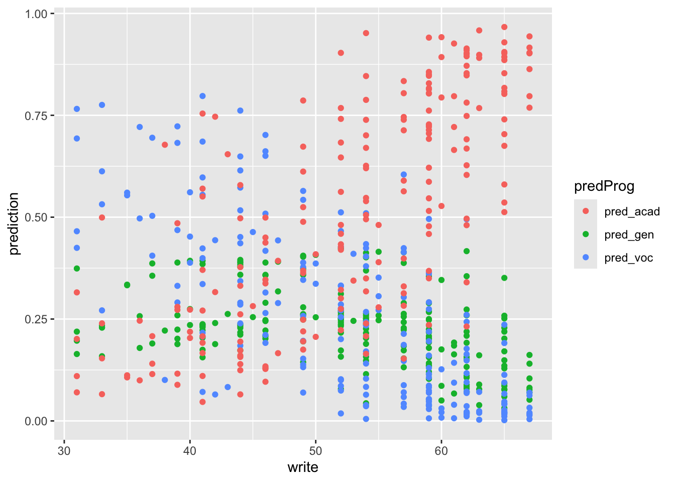

pred_stud_long %>%
  ggplot() +
  geom_boxplot(aes(ses, prediction, color = ses)) +
  facet_wrap(~predProg)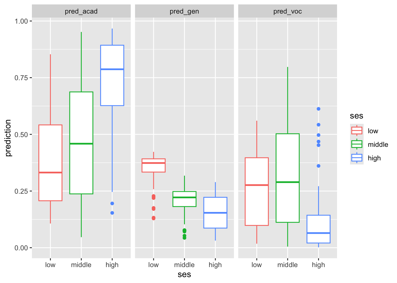

7.6 Other tests

The models fitted so fare are not the only one that can give insights on the data. Here’s some other models and tests made with arbitrary data. Feel free to further experiment the dataset.

# to run this, make sure you have R 4.2 installed.
# otherwise use the alternative way shown in the section above
general_glm <- students |>
  mutate(general = ifelse(prog == "general", 1, 0)) |>
  glm(general ~ ses + schtyp + read + write + math,
    data = _, family = "binomial"
  )
summary(general_glm)

## 
## Call:
## glm(formula = general ~ ses + schtyp + read + write + math, family = "binomial", 
##     data = mutate(students, general = ifelse(prog == "general", 
##         1, 0)))
## 
## Coefficients:
##                Estimate Std. Error z value Pr(>|z|)
## (Intercept)    0.888726   1.139382   0.780    0.435
## sesmiddle     -0.548233   0.411069  -1.334    0.182
## seshigh       -0.787325   0.503662  -1.563    0.118
## schtypprivate -0.050761   0.507839  -0.100    0.920
## read          -0.011416   0.024227  -0.471    0.637
## write          0.009743   0.024416   0.399    0.690
## math          -0.030597   0.027101  -1.129    0.259
## 
## (Dispersion parameter for binomial family taken to be 1)
## 
##     Null deviance: 213.27  on 199  degrees of freedom
## Residual deviance: 205.11  on 193  degrees of freedom
## AIC: 219.11
## 
## Number of Fisher Scoring iterations: 4

general_alt_glm <- students |> # notice no filter on prog != "academic"
  mutate(general = ifelse(prog == "vocation", 1, 0)) |>
  glm(general ~ ses + read + write + math,
    data = _, family = "binomial"
  )
summary(general_alt_glm)

## 
## Call:
## glm(formula = general ~ ses + read + write + math, family = "binomial", 
##     data = mutate(students, general = ifelse(prog == "vocation", 
##         1, 0)))
## 
## Coefficients:
##             Estimate Std. Error z value Pr(>|z|)    
## (Intercept)  6.11922    1.38391   4.422 9.79e-06 ***
## sesmiddle    0.83768    0.45392   1.845   0.0650 .  
## seshigh     -0.12410    0.58500  -0.212   0.8320    
## read        -0.03261    0.02672  -1.220   0.2223    
## write       -0.04151    0.02452  -1.693   0.0904 .  
## math        -0.07799    0.03054  -2.554   0.0107 *  
## ---
## Signif. codes:  0 '***' 0.001 '**' 0.01 '*' 0.05 '.' 0.1 ' ' 1
## 
## (Dispersion parameter for binomial family taken to be 1)
## 
##     Null deviance: 224.93  on 199  degrees of freedom
## Residual deviance: 179.08  on 194  degrees of freedom
## AIC: 191.08
## 
## Number of Fisher Scoring iterations: 5

testdata <- tibble(
  ses = c("low", "middle", "high"),
  write = mean(students$write),
  math = mean(students$math),
  read = mean(students$read)
)
testdata %>%
  mutate(prob = predict(general_alt_glm, newdata = testdata, type = "response"))

## # A tibble: 3 × 5
##   ses    write  math  read  prob
##   <chr>  <dbl> <dbl> <dbl> <dbl>
## 1 low     52.8  52.6  52.2 0.132
## 2 middle  52.8  52.6  52.2 0.261
## 3 high    52.8  52.6  52.2 0.119

testdata <- tibble(
  ses = "low",
  write = c(30, 40, 50),
  math = mean(students$math),
  read = mean(students$read)
)
testdata %>%
  mutate(prob = predict(general_alt_glm, newdata = testdata, type = "response"))

## # A tibble: 3 × 5
##   ses   write  math  read  prob
##   <chr> <dbl> <dbl> <dbl> <dbl>
## 1 low      30  52.6  52.2 0.282
## 2 low      40  52.6  52.2 0.206
## 3 low      50  52.6  52.2 0.146