Chapter 4 The linear model
During this lecture, we will use the Advertising dataset,
which can be found in Kaggle.
It shows, for each line, the revenue (Sales), which is the response depending on
three predictors, i.e. money spent on three different advertising channels: TV, Radio, Newspaper.
Every variable is continuous, allowing to explain the main R
functions used in a plain linear regression task.
4.1 Dataset import
Import the dataset (you may have to select properly the current working directory). Remember a modern version of a dataset in R is called tibble (as opposed to the previous dataframe)
library(readr)
# here the wd contains a folder 'dataset' which
# in turn contains the file to be read
advertising <- read_csv("./datasets/advertising.csv")
## Rows: 200 Columns: 4
## ── Column specification ────────────────────────────────────────────────────────
## Delimiter: ","
## dbl (4): TV, Radio, Newspaper, Sales
##
## ℹ Use `spec()` to retrieve the full column specification for this data.
## ℹ Specify the column types or set `show_col_types = FALSE` to quiet this message.## # A tibble: 200 × 4
## TV Radio Newspaper Sales
## <dbl> <dbl> <dbl> <dbl>
## 1 230. 37.8 69.2 22.1
## 2 44.5 39.3 45.1 10.4
## 3 17.2 45.9 69.3 12
## 4 152. 41.3 58.5 16.5
## 5 181. 10.8 58.4 17.9
## 6 8.7 48.9 75 7.2
## 7 57.5 32.8 23.5 11.8
## 8 120. 19.6 11.6 13.2
## 9 8.6 2.1 1 4.8
## 10 200. 2.6 21.2 15.6
## # ℹ 190 more rows4.2 Basic EDA (Exploratory Data Analysis)
Get some basic statistics with summary()
##        TV             Radio          Newspaper          Sales
##  Min.   :  0.70   Min.   : 0.000   Min.   :  0.30   Min.   : 1.60
##  1st Qu.: 74.38   1st Qu.: 9.975   1st Qu.: 12.75   1st Qu.:11.00
##  Median :149.75   Median :22.900   Median : 25.75   Median :16.00
##  Mean   :147.04   Mean   :23.264   Mean   : 30.55   Mean   :15.13
##  3rd Qu.:218.82   3rd Qu.:36.525   3rd Qu.: 45.10   3rd Qu.:19.05
##  Max.   :296.40   Max.   :49.600   Max.   :114.00   Max.   :27.00
You can attach() the dataset to access columns writing less code, although this is not
recommended nowadays (see with() below). All the columns of the table are then
available in the R environment without prepending the dataset name
## [1] 230.1 44.5 17.2 151.5 180.8 8.7To revert back, detach the dataset
It is better to use with() instead.
This function basically attaches a certain context object
(e.g. the dataset namespace), executes the commands inside
the curly brackets, and then detaches the context object.
## [1] 22.1 10.4 12.0 16.5 17.9  7.2
## [1] 147.0425
##  [1] 10.8 19.6  2.1  2.6  5.8  7.6  5.1 15.9 16.9 12.6  3.5 16.7 16.0 17.4  1.5
## [16]  1.4  4.1  8.4  9.9 15.8 11.7  3.1  9.6 19.2  2.0 15.5  9.3 14.5 14.3  5.7
## [31]  1.6  7.7  4.1 18.4  4.9  1.5 14.0  3.5  4.3 10.1 17.2 11.0  0.3  0.4  8.2
## [46] 15.4 14.3  0.8 16.0  2.4 11.8  0.0 12.0  2.9 17.0  5.7 14.8  1.9  7.3 13.9
## [61]  8.4 11.6  1.3 18.4 18.1 18.1 14.7  3.4  5.2 10.6 11.6  7.1  3.4  7.8  2.3
## [76] 10.0  2.6  5.4  5.7  2.1 13.9 12.1 10.8  4.1  3.7  4.9  9.3  8.6
These are some of the functions that might be useful when gathering information about a dataset.
## [1] 4## [1] 200## [1] 200 4## [1] "TV" "Radio" "Newspaper" "Sales"4.3 Simple plots
When exploring a dataset, ggplot() might be a bit excessive
(recall that ggplot() is a modern way to draw cool plots using
a graphical syntax). Faster plots can be drawn with plot() and pairs()
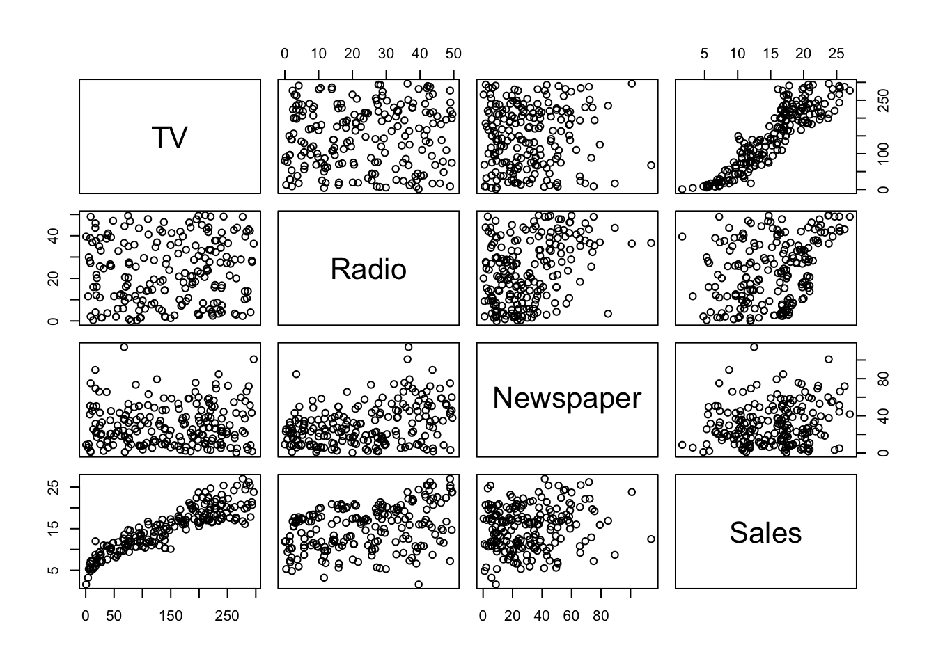
A pair-plot gives a bigger picture of the
cross correlations between variables.
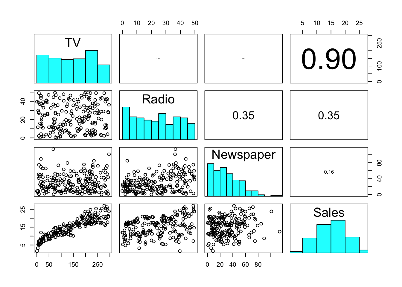
The base R pairs() function can be tweaked (check ?pairs)
in order to draw other kind of information of interest.
## put histograms on the diagonal
panel_hist <- function(x, ...) {
  usr <- par("usr")
  par(usr = c(usr[1:2], 0, 1.5))
  h <- hist(x, plot = FALSE)
  breaks <- h$breaks
  nb <- length(breaks)
  y <- h$counts
  y <- y / max(y)
  rect(breaks[-nb], 0, breaks[-1], y, col = "cyan", ...)
}
## put (absolute) correlations on the upper panels,
## with size proportional to the correlations.
panel_cor <- function(x, y, digits = 2, prefix = "", cex_cor, ...) {
  par(usr = c(0, 1, 0, 1))
  r <- abs(cor(x, y))
  txt <- format(c(r, 0.123456789), digits = digits)[1]
  txt <- paste0(prefix, txt)
  if (missing(cex_cor)) cex_cor <- 0.8 / strwidth(txt)
  text(0.5, 0.5, txt, cex = cex_cor * r)
}

pairs(advertising,
  upper.panel = panel_cor, diag.panel = panel_hist
)
With much less effort, we can obtain a prettier version of the pair-plot.
## Registered S3 method overwritten by 'GGally':
##   method from
##   +.gg   ggplot2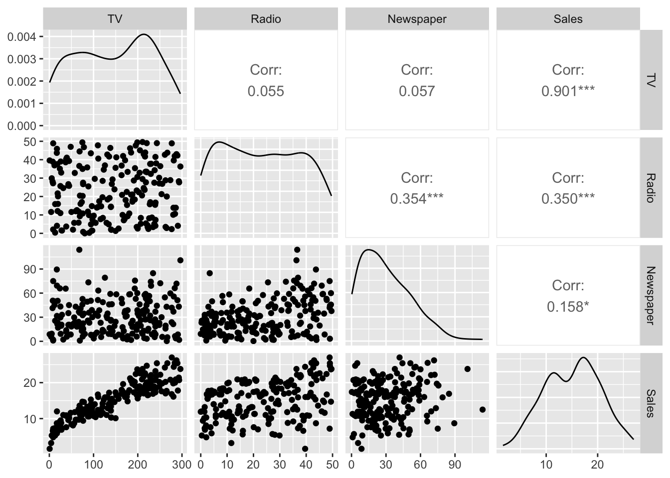
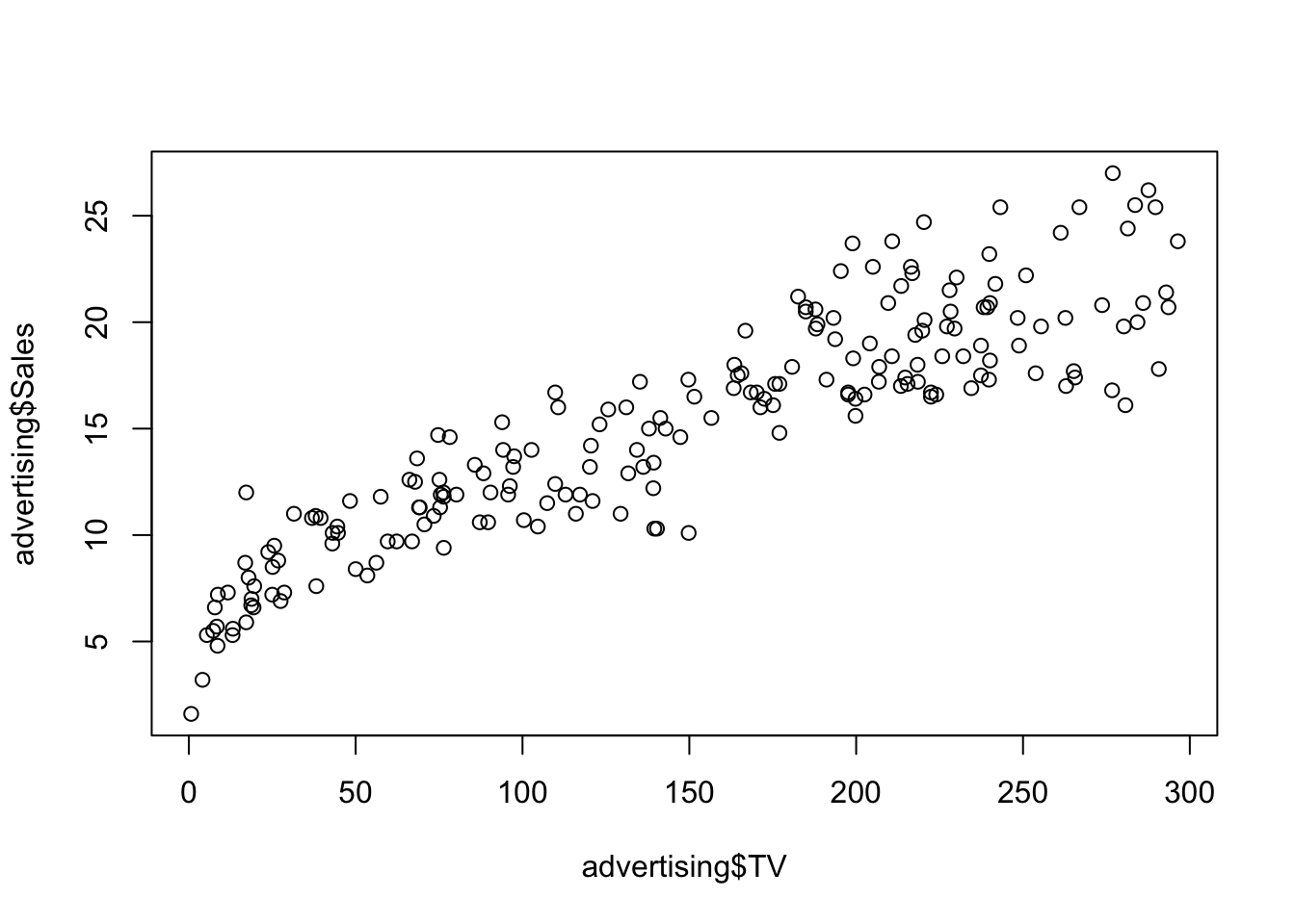
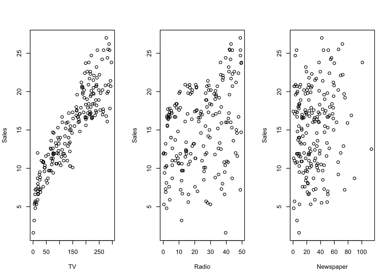
Again, with base R let’s plot the predictors against the response. We know how to do that with a single predictor.
In case we want to add all plots to a single figure, we can do it as follow (base R)
# set plot parameters
with(advertising, {
  par(mfrow = c(1, 3))
  plot(TV, Sales)
  plot(Radio, Sales)
  plot(Newspaper, Sales)
})
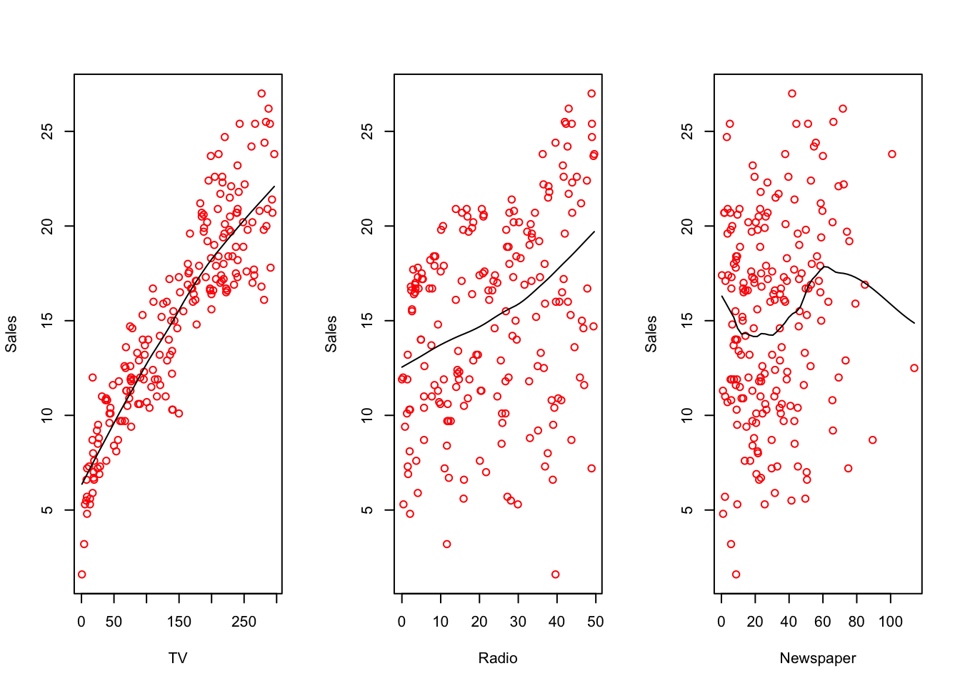
adding a smoothed line would look like this
# set plot parameters
with(advertising, {
  par(mfrow = c(1, 3))
  scatter.smooth(TV, Sales, col = "red")
  scatter.smooth(Radio, Sales, col = "red")
  scatter.smooth(Newspaper, Sales, col = "red", span = .3) # tweak with span
})
The same pictures can also be plotted with ggplot(),
if preferred (in two ways).
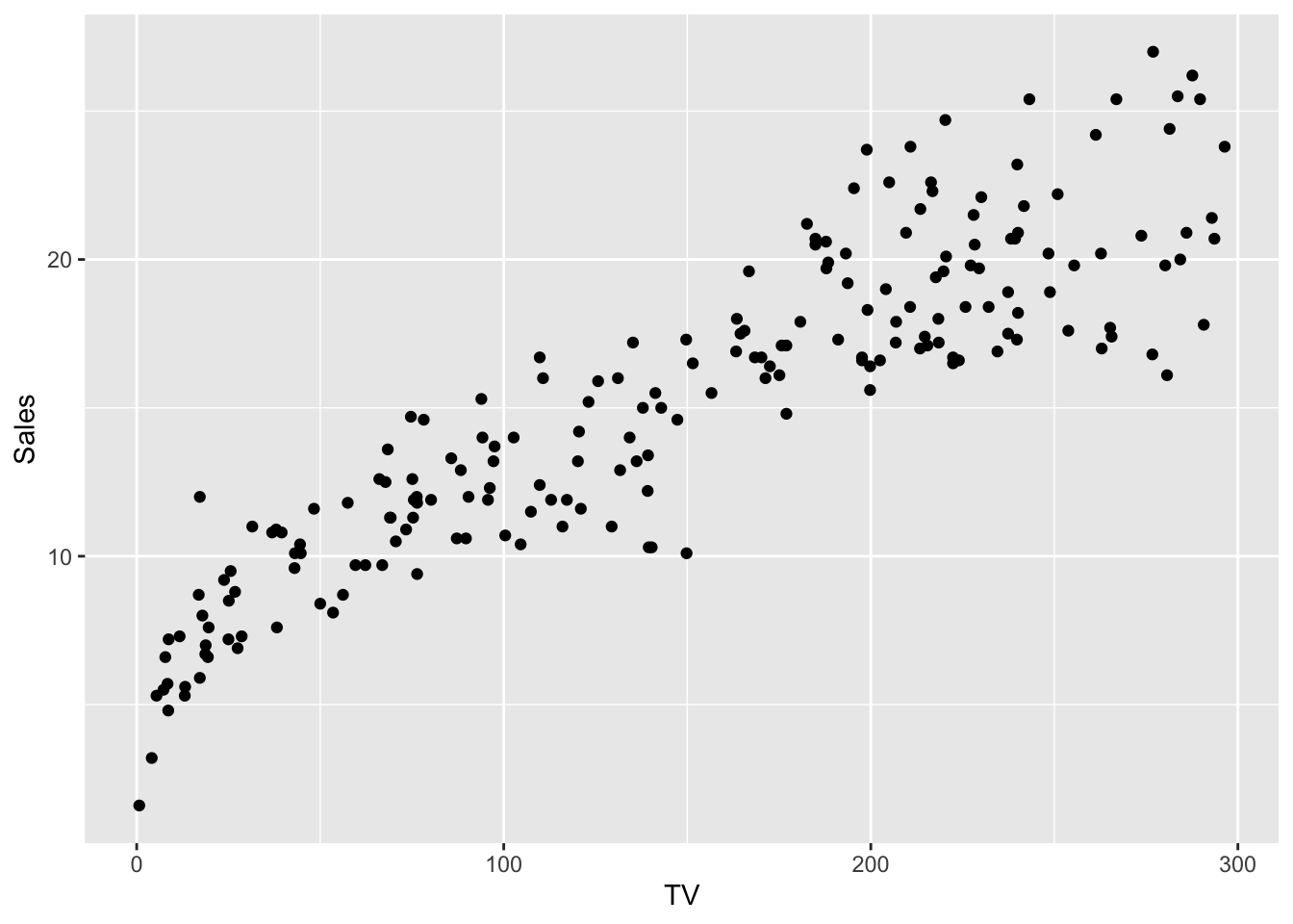
First method: draw three separate plots and arrange
them together with ggarrange()
library(ggpubr)
tvplt <- ggplot(advertising, mapping = aes(TV, Sales)) +
  geom_point() +
  geom_smooth()
radplt <- ggplot(advertising, mapping = aes(Radio, Sales)) +
  geom_point() +
  geom_smooth()
nwsplt <- ggplot(advertising, mapping = aes(Newspaper, Sales)) +
  geom_point() +
  geom_smooth()

ggarrange(tvplt, radplt, nwsplt,
  ncol = 3
)
## `geom_smooth()` using method = 'loess' and formula = 'y ~ x'
## `geom_smooth()` using method = 'loess' and formula = 'y ~ x'
## `geom_smooth()` using method = 'loess' and formula = 'y ~ x'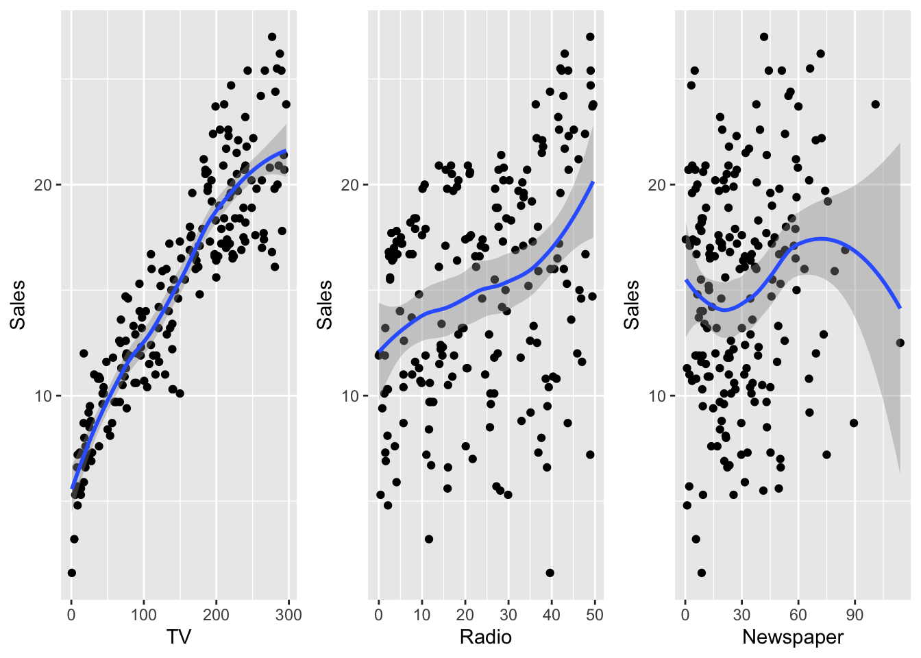
Second method: rearrange the dataset first,
and feed everything to ggplot().
library(tibble)
library(tidyr)

## if using melt, need to switch to data.frame
# library(reshape2)
# advertising <- as.data.frame(advertising)
# long_adv <- melt(advertising, id.vars = "Sales")

long_adv <- advertising %>%
  gather(channel, value, -Sales)
head(long_adv)
## # A tibble: 6 × 3
## Sales channel value
## <dbl> <chr> <dbl>
## 1 22.1 TV 230.
## 2 10.4 TV 44.5
## 3 12 TV 17.2
## 4 16.5 TV 152.
## 5 17.9 TV 181.
## 6 7.2 TV 8.7ggplot(long_adv, aes(value, Sales)) +
geom_point() +
geom_smooth() +
facet_wrap(~channel, scales = "free")## `geom_smooth()` using method = 'loess' and formula = 'y ~ x'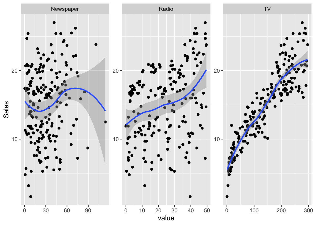
If you’re not sure why we need to use the melt() function,
check the first lab (Iris dataset), or simply read the ?melt
helper.
4.4 Simple regression
The core of this class is the lm() function: its first argument is a formula,
centered around the symbol ~, whith a response on its left and a list of predictors on its right.
Let’s start with a simple single quantitative predictor linear model (simple linear regression)
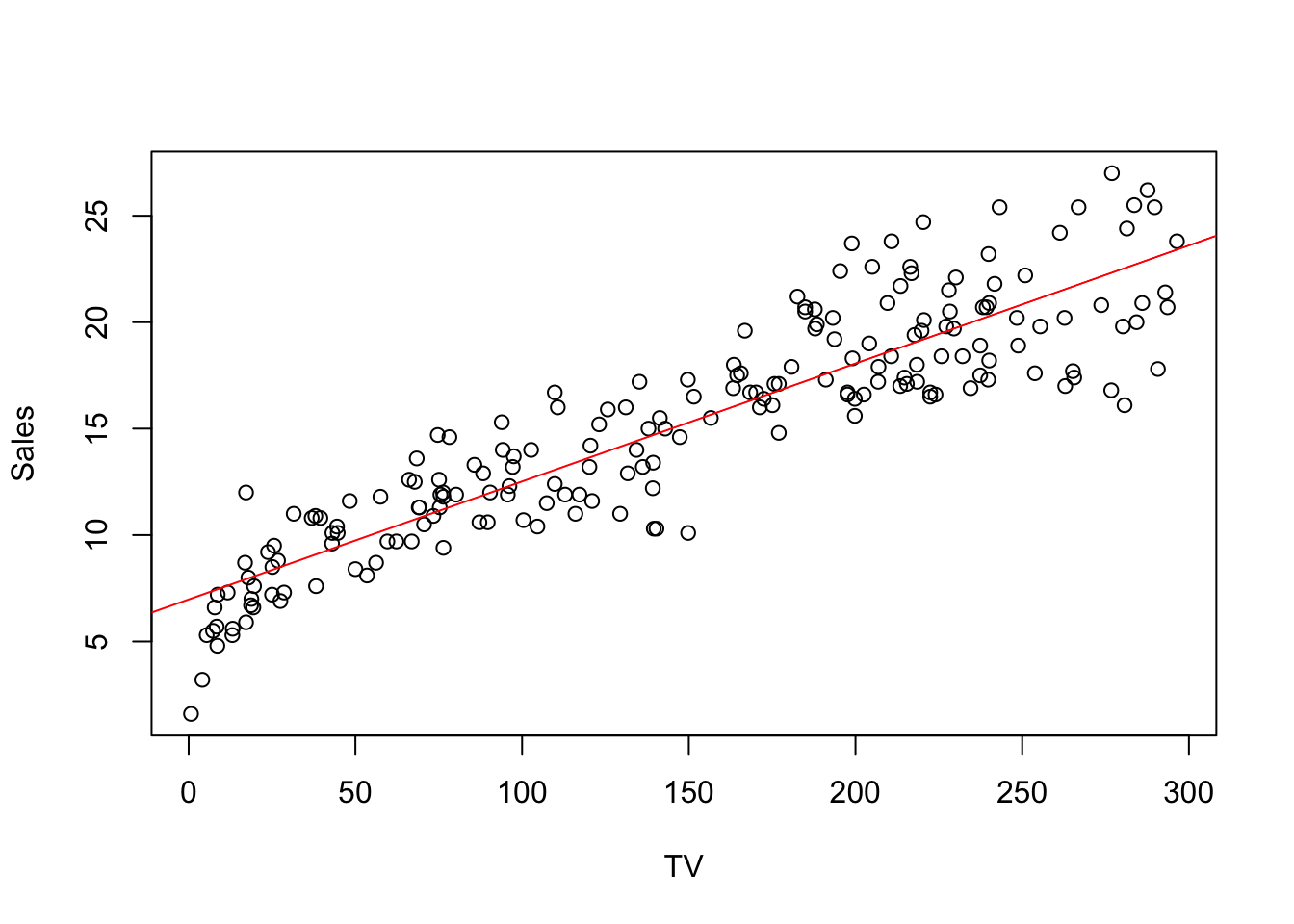
Now that we fitted the model, we have access to the coefficient estimates and we can plot the estimated regression line.
4.4.1 Plot
Here two ways of drawing the regression line, first in base R
with(data = advertising, {
  plot(x = TV, y = Sales)
  # abline draws a line from intercept and slope
  abline(
    simple_reg,
    col = "red"
  )
})
and in ggplot
ggplot(simple_reg, mapping = aes(TV, Sales)) +
  geom_point() +
  geom_smooth(method = "lm", color = "red")
## `geom_smooth()` using formula = 'y ~ x'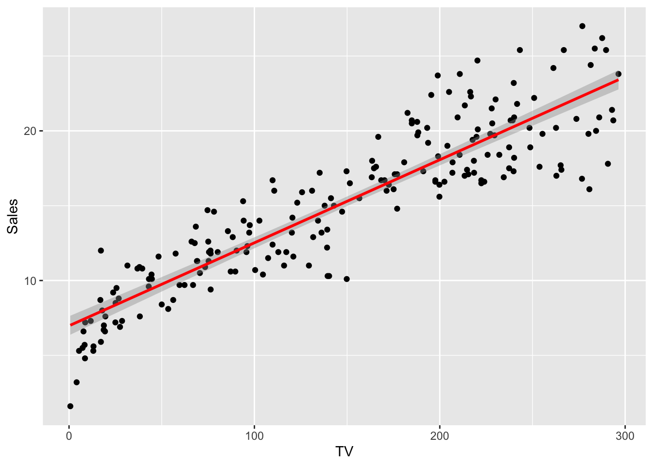
Actually, lm() does a lot more than just compute the least squares coefficients.
##
## Call:
## lm(formula = Sales ~ TV, data = advertising)
##
## Residuals:
##     Min      1Q  Median      3Q     Max
## -6.4438 -1.4857  0.0218  1.5042  5.6932
##
## Coefficients:
##             Estimate Std. Error t value Pr(>|t|)
## (Intercept) 6.974821   0.322553   21.62   <2e-16 ***
## TV          0.055465   0.001896   29.26   <2e-16 ***
## ---
## Signif. codes:  0 '***' 0.001 '**' 0.01 '*' 0.05 '.' 0.1 ' ' 1
##
## Residual standard error: 2.296 on 198 degrees of freedom
## Multiple R-squared:  0.8122, Adjusted R-squared:  0.8112
## F-statistic: 856.2 on 1 and 198 DF,  p-value: < 2.2e-16
We will analyze in detail this output in the next subsection.
4.4.2 Summary
summary(lm) contains information about the following quantities:
residuals: \(Y - X\hat\beta\)
estimated coefficients: \(\hat\beta\)
(estimated) standard errors on the coefficients (in the
Std. Errorcolumn) \(S \sqrt{(X'X)^{-1}_{i+1,i+1}}\) because \(\frac{\hat\beta_i - \beta_i}{S\sqrt{(X'X)^{-1}}}\sim t(n-p)\)in the
t valuecolumn: value of the test statistic for the null hypothesis \(H_0: \beta_{i+1} = 0\)in the
Pr(>|t|)column: p-value regarding the null hypothesis aboveresidual std error: \(S = \sqrt{\frac{e'e}{n-p}}\), i.e. the square root of the Mean Square Residual (MSR)
multiple R squared: later
adj R squared: later
Let’s compute them to make sure we understood the concepts
4.4.2.1 Residuals
Easy to retrieve them (actually, they are the realization of the residuals)
\[ e = y - X\hat\beta \]
y <- advertising$Sales
x <- cbind(1, advertising$TV)
e <- y - x %*% simple_reg$coefficients
head(tibble(
  lm_res = simple_reg$residuals,
  manual_res = as.vector(e)
))
## # A tibble: 6 × 2
## lm_res manual_res
## <dbl> <dbl>
## 1 2.36 2.36
## 2 0.957 0.957
## 3 4.07 4.07
## 4 1.12 1.12
## 5 0.897 0.897
## 6 -0.257 -0.2574.4.2.2 Estimate
Estimates are just the \(\hat\beta\) values for each predictor (plus intercept). They are computed with the closed form max likelihood formula.
\[ \hat\beta = (X'X)^{-1}X'Y \]
beta_hat <- solve(t(x) %*% x) %*% t(x) %*% y
head(tibble(
  lm_coeff = simple_reg$coefficients,
  manual_coeff = as.vector(beta_hat)
))
## # A tibble: 2 × 2
## lm_coeff manual_coeff
## <dbl> <dbl>
## 1 6.97 6.97
## 2 0.0555 0.05554.4.2.3 Standard Error
For each predictor, this quantifies the estimated variation in the beta estimator. The lower the standard error is, the higher is the accuracy of that particular coefficient. For predictor \(i\), it is computed as
\[ SE_i = S \sqrt{(X'X)^{-1}_{i+1,i+1}} \] \(i+1\) is used here since first column if for the intercept \(\beta_0\).
n <- nrow(x)
p <- ncol(x)
rms <- t(e) %*% e / (n - p)

# SE for TV
tv_se <- sqrt(rms * solve(t(x) %*% x)[2, 2])
tv_se
## [,1]
## [1,] 0.0018955514.4.2.4 T-value and p-value
These two are related to each other. The first is the test statistics value, under the null hypothesis \(H_0 : \beta_i = 0\), for the variable
\[ \frac{\hat\beta_i - \beta_i}{S \sqrt{(X'X)^{-1}}} \]
which is student-T distributed with \(n-2\) degrees of freedom.
##         [,1]
## [1,] 29.2605
And finally, the p-value is the probability on a \(t(n-2)\) distribution of the statistic to be beyond the value actually observed. Remember that with beyond we mean on both sides of the distribution, since the alternative hypothesis \(H_1: \beta \neq 0\) is two-sided.
# multiply by two because the alternative hyp is two-sided
p_val <- 2 * pt(t_val, n - 2, lower.tail = FALSE)
p_val
## [,1]
## [1,] 7.927912e-74Here we cannot appreciate the manual computation since the p-value is very low (meaning that we can reject the null, favoring the alternative).
Exercise: You can try to compute this value manually on another
simple regression model where we use Radio as predictor.
##
## Call:
## lm(formula = Sales ~ Radio, data = advertising)
##
## Residuals:
##      Min       1Q   Median       3Q      Max
## -15.5632  -3.5293   0.6714   4.2504   8.6796
##
## Coefficients:
##             Estimate Std. Error t value Pr(>|t|)
## (Intercept)  12.2357     0.6535  18.724  < 2e-16 ***
## Radio         0.1244     0.0237   5.251 3.88e-07 ***
## ---
## Signif. codes:  0 '***' 0.001 '**' 0.01 '*' 0.05 '.' 0.1 ' ' 1
##
## Residual standard error: 4.963 on 198 degrees of freedom
## Multiple R-squared:  0.1222, Adjusted R-squared:  0.1178
## F-statistic: 27.57 on 1 and 198 DF,  p-value: 3.883e-07