Chapter 3 Normal sampling
3.1 Random and non-random normal samples
First we look at the simplest case: independent and identically distributed Normal random variables.
\[ \mathbf{X} \sim \mathcal{N}\left( \begin{pmatrix} \mu \\ \vdots \\ \mu \end{pmatrix}, \begin{pmatrix} \sigma^2 & & & & \\ & & & 0 & \\ & & \ddots & & \\ & 0 & & & \\ & & & & \sigma^2 \end{pmatrix} \right) \]
In order to simulate a sample of i.i.d. Normal r.v.,
we need to call the rnorm function, which uses R pseudo-random number generator.
Like every pseudo-RNG, it allows for specifying a seed, that
is useful for reproducibility purposes
(see pseudo-RNG wiki for
more details).
This is how you can simulate a sample with \(n = 50\) i.i.d. Normal random variables in R.
set.seed(42) # for reproducibility
library(ggplot2) # plotting
library(dplyr) # dataframe manipulation
library(tibble) # tibble

n <- 50
rnorm_sample <- rnorm(n) # mu = 0, sigma = 1, for instance

iidplt <- rnorm_sample %>%
  enframe() %>% # creates tibble with name,value columns
  ggplot() +
  geom_point(aes(x = name, y = value)) +
  labs(title = "Random sample") + # add title and labels to the plot
  xlab("i") +
  ylab("x_i")
iidplt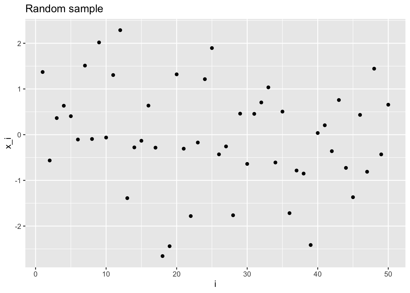
If the random variables are independent but distributed with different mean, we can identify two notable cases: mean shift and mean drift.
In the first case, we write
Mean shift: \[ \mathbf{X} \sim \mathcal{N}\left( \begin{pmatrix} \mu_0 \\ \vdots \\ \mu_0 \\ \mu_1 \\ \vdots \\ \mu_1 \end{pmatrix}, \begin{pmatrix} \sigma^2 & & & & \\ & & & 0 & \\ & & \ddots & & \\ & 0 & & & \\ & & & & \sigma^2 \end{pmatrix} \right)\,, \]
and in R we can simulate such sample as follows
# (optional) creates a function to simplify other plots
plot_sample <- function(x, title = NULL, xlab = NULL, ylab = NULL) {
  plt <- x %>%
    enframe() %>%
    ggplot(aes(x = name, y = value)) +
    geom_point() +
    labs(title = title) +
    xlab(xlab) +
    ylab(ylab)
  return(plt)
}

# first half with mean = 0, second half with mean = 3
# simulate by concatenating two rnorm samples
ms_sample <- c(rnorm(floor(n / 2)), rnorm(n - floor(n / 2), 3))
# or equivalently, by concatenating two mean vectors in one rnorm call
ms_sample <- rnorm(n, mean = c(
  rep(0, floor(n / 2)),
  rep(3, n - floor(n / 2))
))

# save the plot in a variable for later use
msplt <- plot_sample(ms_sample, "Mean-shift", "i", "x_i")
msplt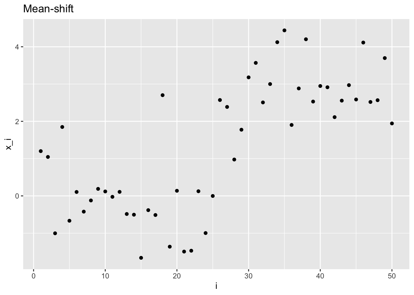
For the mean drift, the mean changes variable by variable
Mean drift: \[ \mathbf{X} \sim \mathcal{N}\left( \begin{pmatrix} \mu_1 \\ \mu_2 \\ \vdots \\ \mu_n \end{pmatrix}, \begin{pmatrix} \sigma^2 & & & & \\ & & & 0 & \\ & & \ddots & & \\ & 0 & & & \\ & & & & \sigma^2 \end{pmatrix} \right)\,, \]
Similarly, in R, we can simulate a mean drift with mean going from \(0\) to \(n-1\) with unitary step.
# mean is a range vector
md_sample <- rnorm(n, 0:(n - 1))

mdplt <- plot_sample(md_sample, "Mean drift", "i", "x_i")
mdplt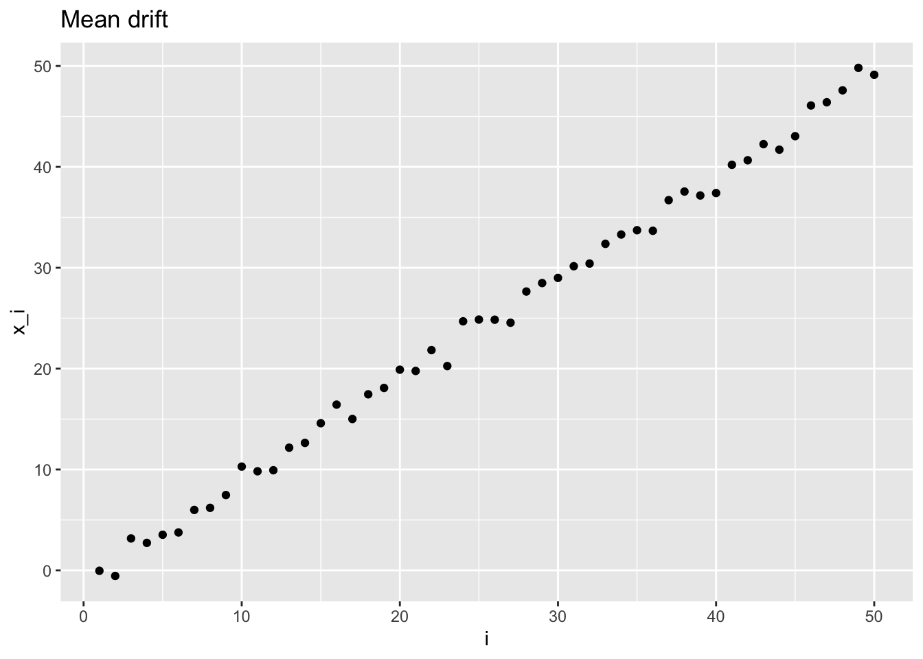
The same concept is applied also to random variables drawn by a normal with changing variance.
Variance shift: \[ \mathbf{X} \sim \mathcal{N}\left( \begin{pmatrix} \mu \\ \vdots \\ \mu \end{pmatrix}, \begin{pmatrix} \sigma_0^2 & & & & & \\ & \ddots & & & 0 & \\ & & \sigma_0^2 & & & \\ & & & \sigma_1^2 & & \\ & 0 & & & \ddots & \\ & & & & & \sigma_1^2 \end{pmatrix} \right)\,, \]
in R:
vs_sample <- c(
  rnorm(floor(n / 2)), # first half
  rnorm(n - floor(n / 2), sd = 4)
) # second half

vsplt <- plot_sample(vs_sample, "Variance shift", "i", "x_i")
vsplt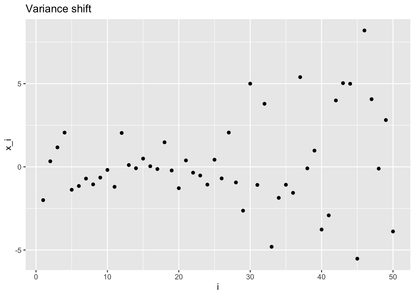
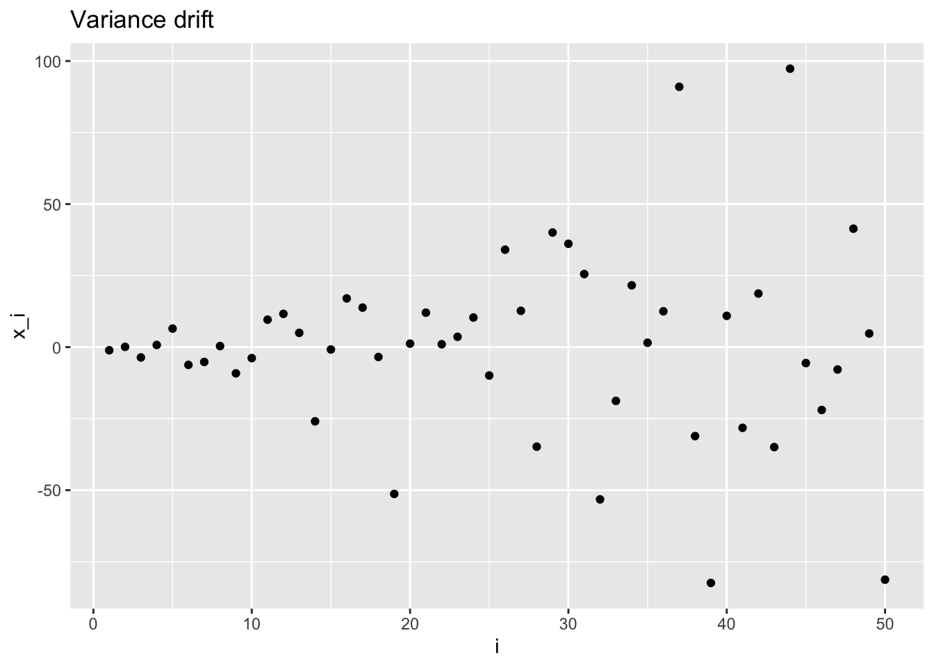
Variance drift
\[ \mathbf{X} \sim \mathcal{N}\left( \begin{pmatrix} \mu \\ \vdots \\ \mu \end{pmatrix}, \begin{pmatrix} \sigma_1^2 & & & & \\ & & & 0 & \\ & & \ddots & & \\ & 0 & & & \\ & & & & \sigma_n^2 \end{pmatrix} \right)\,, \]
in R:
3.1.1 Autocorrelated sample
Let \(\mathbf{Y} = Y_1, ..., Y_{n+1}\) an i.i.d. standard Normal random sample (i.e. \(Y_i \sim \mathcal{N}(0, 1)\)).
Then \(\mathbf{X} = X_1, ..., X_n\) such that \(X_i = Y_{i+1} - Y_i\) is a Normal non-random sample with such distribution
\[ \mathbf{X} \sim \mathcal{N}\left( \begin{pmatrix} 0 \\ \vdots \\ 0 \end{pmatrix}, \begin{pmatrix} 2 & -1 & & & \\ -1 & 2 & & 0 & \\ & & & & \\ & \ddots & \ddots & \ddots & \\ & & & & \\ & 0 & & 2 & -1 \\ & & & -1 & 2 \end{pmatrix} \right)\,. \]
The proof is left as exercise to the reader.
Hint: first compute \(E[X_i]\), then \(\text{Var}(X_i)\) and finally \(\text{Cov}(X_{i+1}, X_i)\)
In R, we build this simulation by simulating \(\mathbf Y\) and deriving \(\mathbf X\)
y <- rnorm(n)
# index by removing first and last elements
auto_sample <- y[-1] - y[-n]
# equivalent to
auto_sample <- y[2:n] - y[1:(n - 1)]
or, simpler
##  [1]  0.76486294 -0.72125125  0.69608123 -0.88154477  0.08858529  0.54025680
##  [7]  0.51057417 -2.23933913  1.21290797 -0.03747466 -0.68795847 -0.27543871
## [13]  0.40362741  1.21753967 -1.00313038 -0.36856515  0.94830413 -1.40013055
## [19]  2.28258801 -1.53046919  0.67372423 -0.13812248 -0.05124700  1.80962271
## [25] -2.63471000  1.97079841 -1.11389726 -0.86677899  0.76644216  0.81553534
## [31] -1.17229042 -0.34656350  0.92484634  0.83583274 -1.06205518 -1.31356822
## [37]  0.08035065  0.53828058  0.24128720  0.50568106  0.69192514 -1.10511511
## [43] -0.67926274  1.72098578 -0.33164903  0.88189010 -2.83982793  1.76979995
## [49]  1.26604281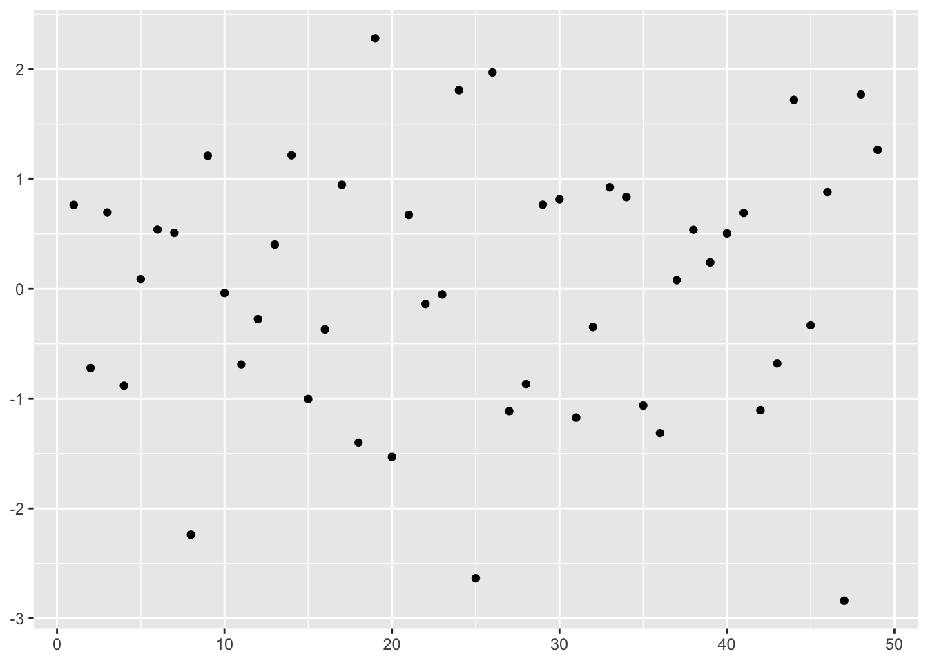
From this plot it is almost impossible to spot the correlation between variables. It’s more visible with a plot having \(X_i\) on one axis and \(X_{i+1}\) on the other.
autoplt <- auto_sample %>%
  { # group in curly brackets so that tibble is called
    # without passing auto_sample as first implicit argument
    tibble(x = .[-length(.)], y = .[-1]) # dot as placeholder
    # equivalent (but more efficient) to:
    # tibble(x = auto_sample[-length(auto_sample)], y = auto_sample[-1])
  } %>%
  ggplot() +
  geom_point(aes(x, y)) +
  labs(title = "autocorrelation") +
  xlab("x_i") +
  ylab("x_{i+1}")
autoplt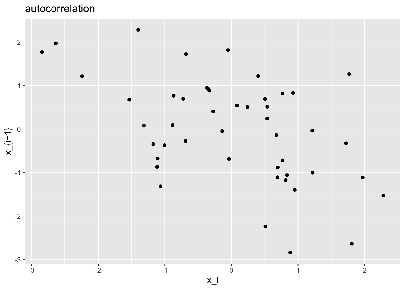
Maybe it’s even more clear if the number of observations increases. Try with larger n.
Questions:
- how is \(X_i\) distributed?
- what is the correlation between two subsequent samples i.e. \(\rho(X_{i+1}, X_{i})\)
Exercise: build Xpos such that correlation is positive
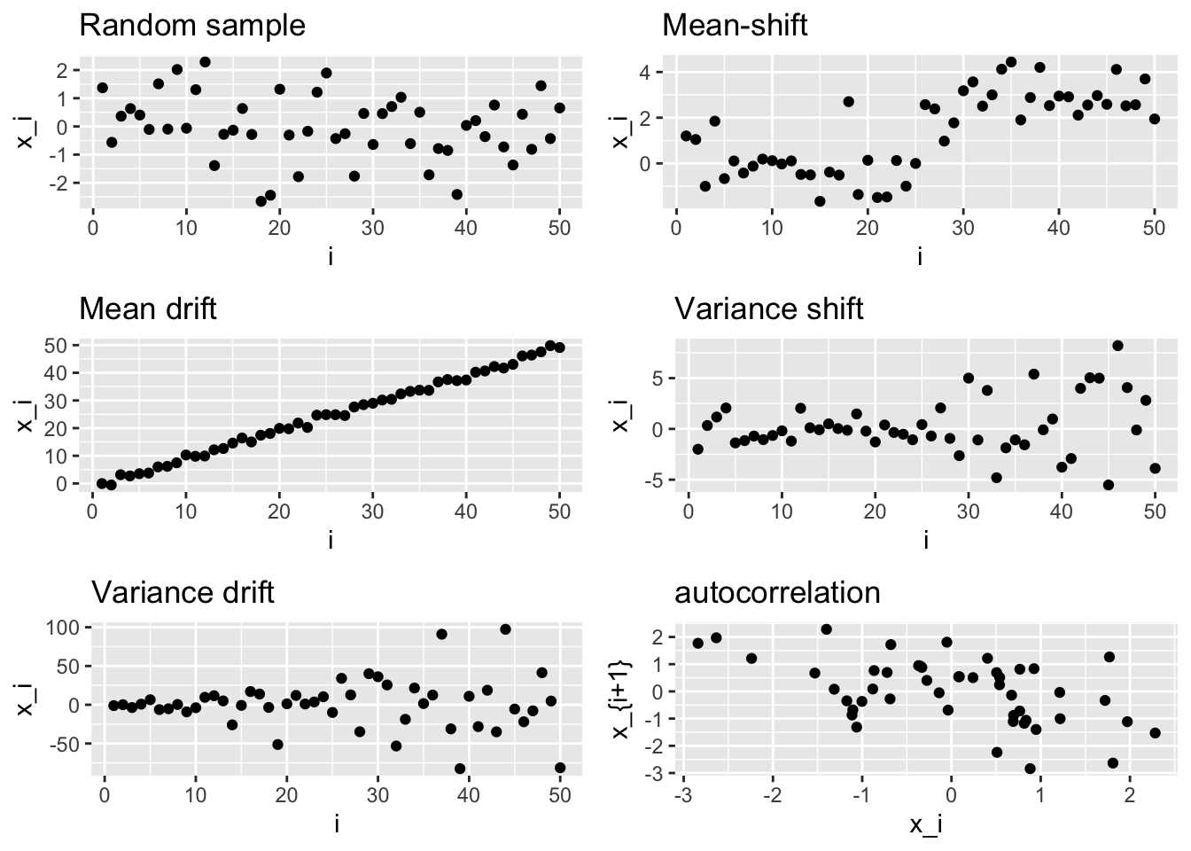
We can compare these models by grouping all the plots in one single picture.
# install.packages("ggpubr")
library(ggpubr)
ggarrange(iidplt, msplt, mdplt, vsplt, vdplt, autoplt,
  nrow = 3, ncol = 2
)
3.2 Exchangeable normal random variables
Let \(\mathbf{X} = (X_1, ..., X_n)\) be a random vector whose elements follow the conditional distribution \[ X_i | \mu \sim \mathcal{N}(\mu, \sigma^2) \] with \(\mu\) being another normally distributed r.v. \[ \mu \sim \mathcal{N}(\mu_0, \sigma_0^2)\,. \]
\(X_i\) are conditionally independent given \(\mu\), and also, their joint distribution is equal for any permutation of the random vector elements (exchangeable). But if we don’t know \(\mu\), what is the distribution of \(X_i\) (marginal distribution)?
It’s
\[ \mathbf{X} \sim \mathcal{N}\left(\begin{pmatrix} \mu_0 \\ \vdots \\ \mu_0 \end{pmatrix}, \begin{pmatrix} \sigma^2 + \sigma_0^2 & & & & \\ & \ddots & & \sigma_0^2 & \\ & & \ddots & & \\ & \sigma_0^2 & & \ddots & \\ & & & & \sigma^2 + \sigma_0^2 \end{pmatrix} \right) \]
Exercise: prove it (i.e. find expected value, variance and covariance).
Hint: \(E[X_i] = E_{f\sim \mu}[E_{f\sim X_i | \mu}[X_i | \mu]]\)
In R, we simply simulate a realization of the mean r.v., then use that value to simulate the \(\mathbf X\) Normal sample given \(\mu\).
3.3 Multivariate Normal random samples
Multivariate normal distribution functions are provided by the mvtnorm library.
Take this as an example:
\[ \begin{pmatrix} X \\ S \end{pmatrix} \sim \mathcal{N} \left( \begin{pmatrix} 0 \\ 0 \end{pmatrix}, \begin{pmatrix} 1 & 1 \\ 1 & 3 \end{pmatrix} \right) \]
# install.packages("mvtnorm")
library(mvtnorm)

# simulate n bivariate normal r.v.
m <- rep(0, 2) # mean vector
vcov_mat <- matrix(c(1, 1, 1, 3), nrow = 2) # Sigma

# specify mean vector and var-cov matrix
bvt_samples <- mvtnorm::rmvnorm(n, m, vcov_mat)
head(bvt_samples, 10) # print only the first 10 elements
## [,1] [,2]
## [1,] -0.78186845 -0.2389248
## [2,] -0.17599524 -0.9582082
## [3,] -0.92364519 -0.3863103
## [4,] 1.17077708 2.7456040
## [5,] -2.03263913 -1.9171945
## [6,] -0.92418665 -2.9286612
## [7,] -0.99088212 -1.6003554
## [8,] -1.50519809 -3.9739964
## [9,] -0.04465341 -0.9858018
## [10,] 1.70934985 1.9264325Let’s plot this sample
bvt_samples_df <- tibble(x = bvt_samples[, 1], s = bvt_samples[, 2])
bvt_scatter <- bvt_samples_df %>%
  ggplot() +
  geom_point(aes(x, s)) +
  coord_fixed(xlim = c(-3, 3), ylim = c(-5, 5), ratio = -.7)

bvt_scatter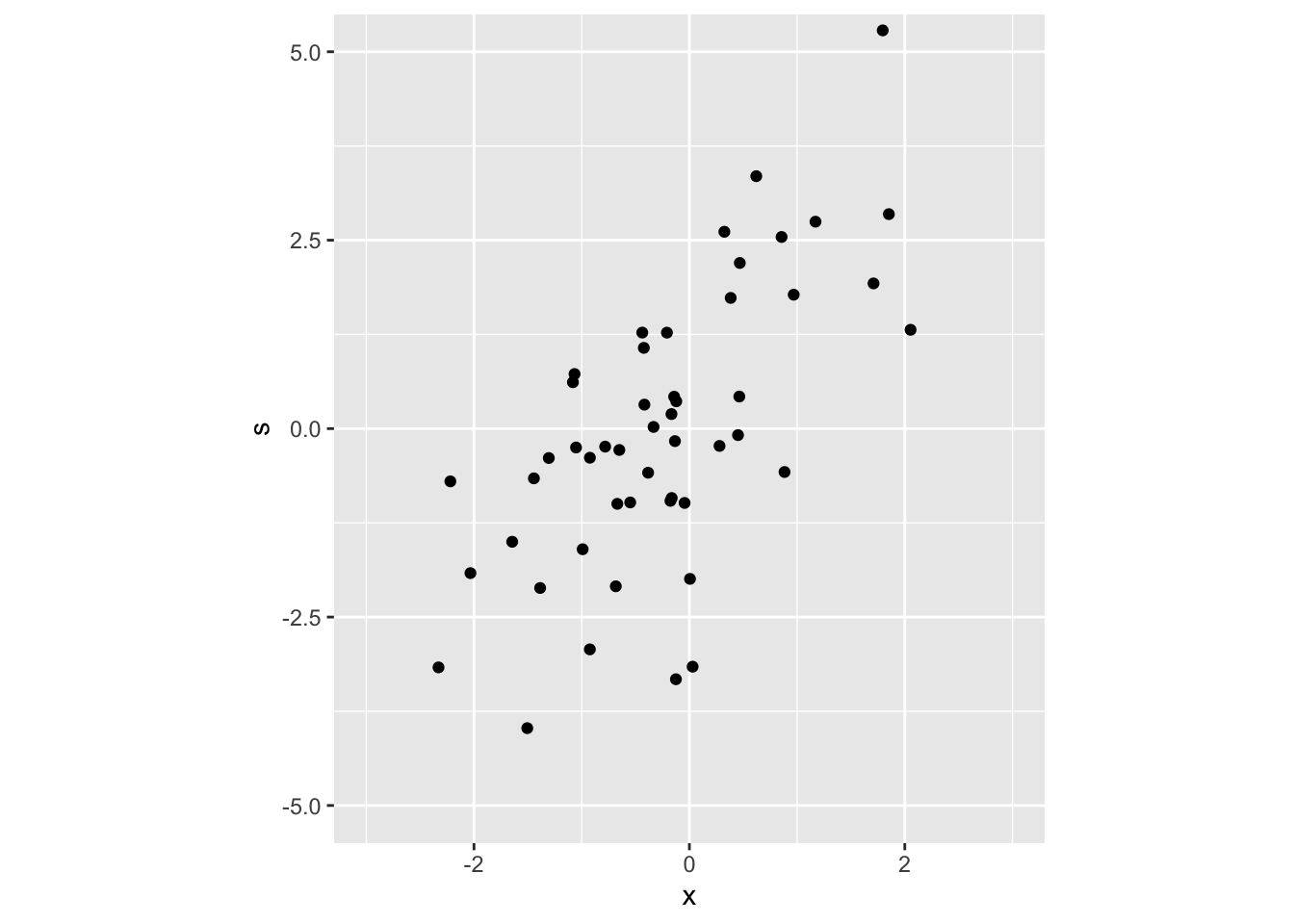
# plot the true distribution
# generate a grid (many points with fixed space between them)
bvt_grid <- expand.grid(
  x = seq(-3, 3, length.out = 200), # seq builds a sequence vector starting from
  # 3 until 3 with step such that the number of elements in the vector is 200
  s = seq(-4, 4, length.out = 200)
)

# compute the density at each coordinate of the grid
probs <- dmvnorm(bvt_grid, m, vcov_mat)
bvt_grid %>%
  mutate(prob = probs) %>% # add a column (?dplyr::mutate)
  ggplot() +
  geom_contour(aes(x, s, z = prob)) + # or geom_contour_filled
  coord_fixed(xlim = c(-3, 3), ylim = c(-5, 5), ratio = -.7)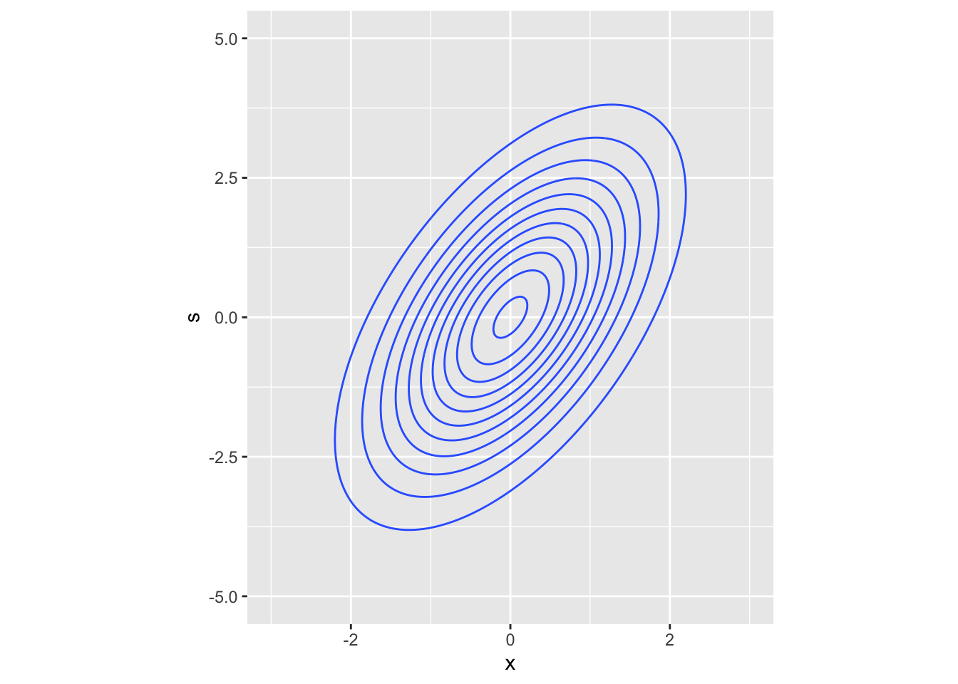
3.3.1 Exercises
Take two bivariate random variables (the same as before, \(X, S\)). Complete these tasks:
- Compute \(P(X < 0 \cap S < 0)\) with
pmvnorm - Compute \(P(X < 0 \cap S< 0)\) by simulation (Monte Carlo estimate)
- Compute \(P(X > 1 \cap S < 0)\) by simulation. Can you do it with
pmvnorm? (hint: check?pmvnorm)
3.3.2 Solutions
## [1] 0.3479566
## attr(,"error")
## [1] 1e-15
## attr(,"msg")
## [1] "Normal Completion"
sim <- rmvnorm(100000, mean = m, sigma = vcov_mat) # simulate enough samples
# count all the observations satisfying the condition
# and divide by the number of total obs to obtain a ratio
# mean() applied to logical values is the proportion of true vars
mean(sim[, 1] < 0 & sim[, 2] < 0)## [1] 0.34856## [1] 0.0238# use lower and upper limits as described in the pmvnorm docs
pmvnorm(lower = c(1, -Inf), upper = c(Inf, 0), mean = m, sigma = vcov_mat)## [1] 0.0240375
## attr(,"error")
## [1] 1e-15
## attr(,"msg")
## [1] "Normal Completion"Increasing the Monte Carlo samples you will get a more accurate estimate of the probability measure.