Chapter 10 Three JAGS examples

10.1 Rats - Simple linear regression

We use the data from (Gelfand et al. 1990) and select the 9th observation which features the weight at 5 different time points of a single rat.

We estimate the intercept and the coefficient in a Bayesian framework using JAGS, then validate our result with the traditional lm. This example is taken from (Lunn et al. 2013)

set.seed(101)
# load data
# install.packages("R2MLwiN")

data(rats, package = "R2MLwiN")
y <- unlist(rats[9, 1:5])
x <- c(8, 15, 22, 29, 36)

library(R2jags)

## Loading required package: rjags

## Loading required package: coda

## Linked to JAGS 4.3.2

## Loaded modules: basemod,bugs

## 
## Attaching package: 'R2jags'

## The following object is masked from 'package:coda':
## 
##     traceplot

model_code <- "
model {
  for (i in 1:5) {
    y[i] ~ dnorm(mu[i], tau)
    mu[i] <- alpha + beta*x[i]
  }

  alpha ~ dnorm(0, 10^-5)
  beta ~ dnorm(0, 10^-5)
  tau ~ dgamma(0.0001, 0.0001)
  sigma2 <- 1 / tau
}
"
model_data <- list(y = y, x = x)
model_params <- c("alpha", "beta", "sigma2")
model_run <- jags(
  data = model_data,
  parameters.to.save = model_params,
  model.file = textConnection(model_code),
  n.chains = 2, n.burnin = 500, n.iter = 5000
)

## module glm loaded

## Compiling model graph
##    Resolving undeclared variables
##    Allocating nodes
## Graph information:
##    Observed stochastic nodes: 5
##    Unobserved stochastic nodes: 3
##    Total graph size: 31
## 
## Initializing model

model_run$BUGSoutput

## Inference for Bugs model at "4", fit using jags,
##  2 chains, each with 5000 iterations (first 500 discarded), n.thin = 4
##  n.sims = 2250 iterations saved
##           mean     sd 2.5%   25%   50%   75%  97.5% Rhat n.eff
## alpha    123.5   19.8 85.6 114.3 123.7 132.3  160.9    1  1000
## beta       7.3    0.8  5.8   7.0   7.3   7.7    8.9    1  2200
## deviance  39.9    3.8 35.8  37.2  38.9  41.6   49.5    1  2200
## sigma2   450.8 3223.0 40.2  87.5 153.9 294.9 2028.3    1  2200
## 
## For each parameter, n.eff is a crude measure of effective sample size,
## and Rhat is the potential scale reduction factor (at convergence, Rhat=1).
## 
## DIC info (using the rule, pD = var(deviance)/2)
## pD = 7.2 and DIC = 47.2
## DIC is an estimate of expected predictive error (lower deviance is better).

library(tibble)

lmfit <- lm(y ~ x, data = tibble(x = x, y = y))
summary(lmfit)

## 
## Call:
## lm(formula = y ~ x, data = tibble(x = x, y = y))
## 
## Residuals:
##     1     2     3     4     5 
##  -5.4   2.4   0.2  14.0 -11.2 
## 
## Coefficients:
##             Estimate Std. Error t value Pr(>|t|)    
## (Intercept) 123.8857    11.8788   10.43 0.001882 ** 
## x             7.3143     0.4924   14.86 0.000662 ***
## ---
## Signif. codes:  0 '***' 0.001 '**' 0.01 '*' 0.05 '.' 0.1 ' ' 1
## 
## Residual standard error: 10.9 on 3 degrees of freedom
## Multiple R-squared:  0.9866, Adjusted R-squared:  0.9821 
## F-statistic: 220.7 on 1 and 3 DF,  p-value: 0.000662

We obtain same values for \(\alpha\) (intercept) and \(\beta\) (slope).

10.2 ZIP model

We generate some synthetic data according to a set of pre-defined parameters (\(p, \lambda\)).

library(ggplot2)

n <- 100
pp <- .3 # probability of zero event
ll <- 5
zi_sample <- rbinom(n, 1, 1 - pp)
zi_sample[zi_sample == 1] <- rpois(sum(zi_sample), lambda = ll) # sample poisson

tibble(y = zi_sample) %>%
  ggplot() +
  geom_histogram(aes(y))

## `stat_bin()` using `bins = 30`. Pick better value with `binwidth`.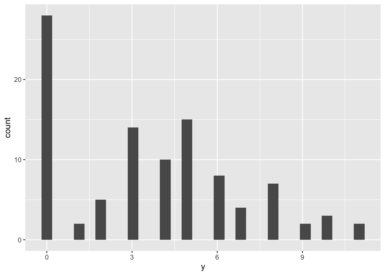

model_code <- "
model {
  for (i in 1:N) {
    y[i] ~ dpois(m[i])
    m[i] <- group[i] * mu
    group[i] ~ dbern(p)
  }

  p ~ dunif(0, 1) # probability of y being drawn from a Poisson
  mu ~ dgamma(0.5, 0.0001)
}
"

model_data <- list(y = zi_sample, N = n)
model_params <- c("mu", "p")
model_run <- jags(
  data = model_data,
  parameters.to.save = model_params,
  model.file = textConnection(model_code),
  n.chains = 2, n.burnin = 500, n.iter = 2000
)

## Compiling model graph
##    Resolving undeclared variables
##    Allocating nodes
## Graph information:
##    Observed stochastic nodes: 100
##    Unobserved stochastic nodes: 102
##    Total graph size: 307
## 
## Initializing model

model_run$BUGSoutput

## Inference for Bugs model at "5", fit using jags,
##  2 chains, each with 2000 iterations (first 500 discarded)
##  n.sims = 3000 iterations saved
##           mean  sd  2.5%   25%   50%   75% 97.5% Rhat n.eff
## deviance 329.0 6.9 323.5 323.8 324.9 334.0 345.2    1  3000
## mu         5.1 0.3   4.6   5.0   5.1   5.3   5.7    1  1600
## p          0.7 0.0   0.6   0.7   0.7   0.8   0.8    1  1000
## 
## For each parameter, n.eff is a crude measure of effective sample size,
## and Rhat is the potential scale reduction factor (at convergence, Rhat=1).
## 
## DIC info (using the rule, pD = var(deviance)/2)
## pD = 24.1 and DIC = 353.1
## DIC is an estimate of expected predictive error (lower deviance is better).

Check that: - the true values fall inside the 95% CI - Rhat is close to 1 (chain convergence)

10.3 Gaussian Mixture Model (GMM)

GMMs are used for clustering data, i.e. group observations which are similar and come from a Gaussian with same mean. It is called mixture in that every observation comes from a Gaussian with a certain mean, and the mean depends in turn on the component/cluster to which it belongs. Therefore the mean is a random variable selected among multiple means (Categorical distributed).

Other mixture models are the ZIP model (mixture of a Poisson and a Bernoulli distribution) and the Negative Binomial (mixture of a Poisson and a Gamma - details).

We generate a sample from a GMM with just two components, arbitrarily defining the true parameters.

# synthetic dataset
n <- 500
group_prob <- .2
means <- c(4., 9.)
stdev <- 2 # same sd for simplicity

# sample the component to which the observation
mixt_groups <- rbinom(n, 1, group_prob) # bernoulli trials
# sample the Gaussian variable setting the mean
# equal to means[1] or means[2] depending on the
# group to which each observation belongs
mixt_sample <- rnorm(n,
  mean = unlist(lapply(mixt_groups, FUN = function(g) means[g + 1])),
  sd = stdev
)

# plot the data
tibble(y = mixt_sample) %>%
  ggplot() +
  geom_histogram(aes(y), binwidth = 0.4)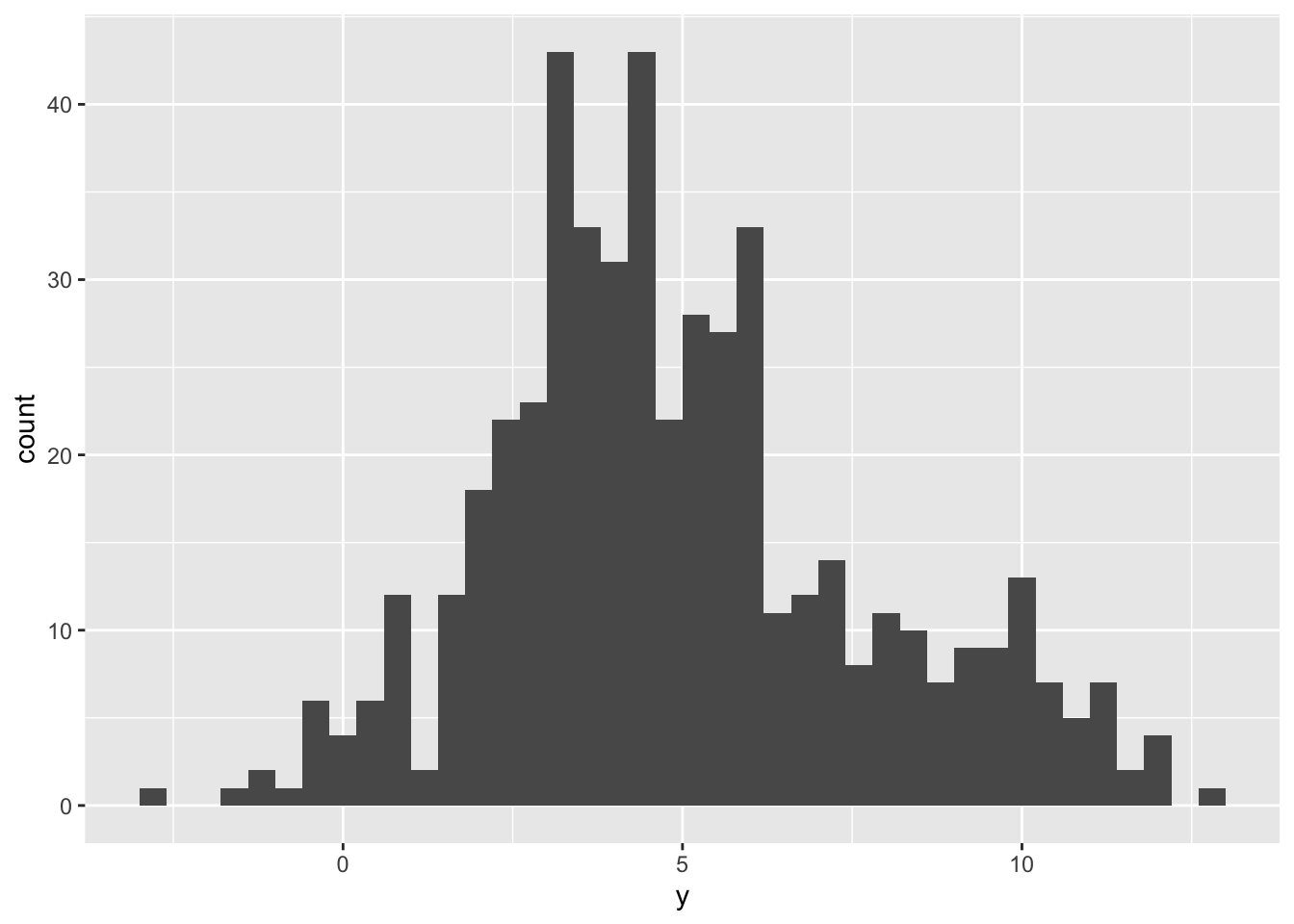

model_code <- "
model {
  for(i in 1:N) {
    y[i] ~ dnorm(mu[i] , tau)
    mu[i] <- mu_clust[clust[i] + 1]
    clust[i] ~ dbern(gp)
  }

  # priors
  gp ~ dbeta(1, 1) # uniform prior
  tau ~ dgamma(0.01, 0.01)
  sigma <- sqrt(1/tau)

  mu_clust_raw[1] ~ dnorm(0, 10^-2)
  mu_clust_raw[2] ~ dnorm(0, 10^-2)

  mu_clust <- sort(mu_clust_raw) # ensure order to prevent label switch
}
"

model_data <- list(y = mixt_sample, N = n)
# save the parameters and, optionally, the
# `clust` variable representing the labeling
# of each observation (clust[i] = 1 if y[i] is found
# to belong to the second cluster, 0 otherwise)
model_params <- c(
  "mu_clust", "gp", "sigma"
  # , "clust"
)
model_run <- jags(
  data = model_data,
  parameters.to.save = model_params,
  model.file = textConnection(model_code),
  n.chains = 2, n.burnin = 1000, n.iter = 5000
)

## Compiling model graph
##    Resolving undeclared variables
##    Allocating nodes
## Graph information:
##    Observed stochastic nodes: 500
##    Unobserved stochastic nodes: 504
##    Total graph size: 2018
## 
## Initializing model

model_run$BUGSoutput

## Inference for Bugs model at "6", fit using jags,
##  2 chains, each with 5000 iterations (first 1000 discarded), n.thin = 4
##  n.sims = 2000 iterations saved
##               mean   sd   2.5%    25%    50%    75%  97.5% Rhat n.eff
## deviance    2066.9 33.3 2009.2 2043.6 2062.9 2087.4 2138.1    1  2000
## gp             0.2  0.0    0.2    0.2    0.2    0.2    0.3    1  1700
## mu_clust[1]    4.0  0.1    3.7    3.9    4.0    4.0    4.2    1  1900
## mu_clust[2]    9.0  0.3    8.4    8.8    9.0    9.2    9.6    1   330
## sigma          1.9  0.1    1.8    1.9    1.9    2.0    2.1    1  2000
## 
## For each parameter, n.eff is a crude measure of effective sample size,
## and Rhat is the potential scale reduction factor (at convergence, Rhat=1).
## 
## DIC info (using the rule, pD = var(deviance)/2)
## pD = 555.0 and DIC = 2621.9
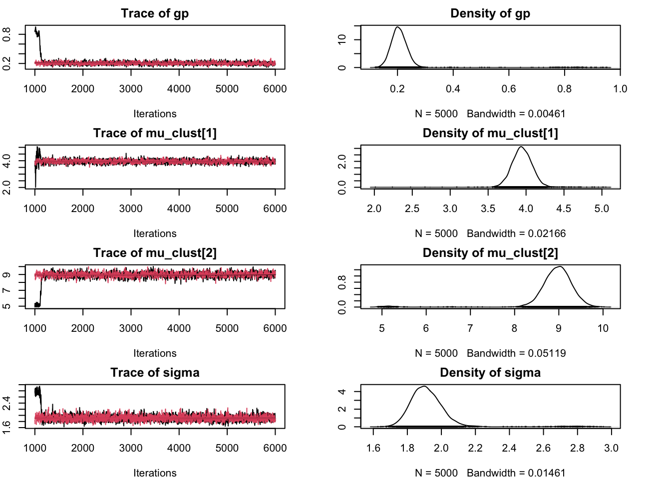
## DIC is an estimate of expected predictive error (lower deviance is better).

We can plot the chain samples in order to verify that the components correctly represent the two clusters.

library(coda)
jags_model <- jags.model(
  file = textConnection(model_code),
  data = model_data,
  n.chains = 2,
  n.adapt = 1000
)

## Compiling model graph
##    Resolving undeclared variables
##    Allocating nodes
## Graph information:
##    Observed stochastic nodes: 500
##    Unobserved stochastic nodes: 504
##    Total graph size: 2018
## 
## Initializing model

samps <- coda.samples(jags_model, model_params, n.iter = 5000)
par(mar = c(4, 2, 2, 4)) # correct plot size
plot(samps)

References

Gelfand, Alan E., Susan E. Hills, Amy Racine-Poon, and Adrian F. M. Smith. 1990. “Illustration of Bayesian Inference in Normal Data Models Using Gibbs Sampling.” Journal of the American Statistical Association 85 (412): 972–85. https://doi.org/10.1080/01621459.1990.10474968.

Lunn, David, Christopher Jackson, Nicky Best, Andrew Thomas, and D. J. Spiegelhalter. 2013. The BUGS Book: A Practical Introduction to Bayesian Analysis. Boca Raton: CRC Press, Taylor & Francis Group.